Get in touch with Zejiang Paper Machinery Company


Updated November 2026
PID tuning means choosing the proportional, integral and derivative settings of a controller so a loop reaches its setpoint without cycling. For self-regulating process loops, a practical way to usable settings is a valve check, a bump test and a lambda calculation.
Paper machines impose another restriction that general tutorials skip. ABB engineers Murphy and Starr expect stock flow to settle within 30 to 80 seconds of a setpoint change, and headbox total head within 50 to 160 seconds. Those loops also influence one another, so the rate of one loop controls how quickly the next one can reach a setpoint. Drones, 3D printers and servo drives use PID control too, but their motion and heater loops have different dynamics; this tutorial covers industrial process loops.
Key points
- Lambda tuning is widely used on paper machines because it allows you to specify the individual speed for each loop.
- As a good initial rule of thumb, a cascade inner loop runs at least 5x faster than the outer loop.
- Between 20 and 30% of paper mill loops were reported to oscillate because of valve problems, which no gain change can repair.
What Is PID Tuning?
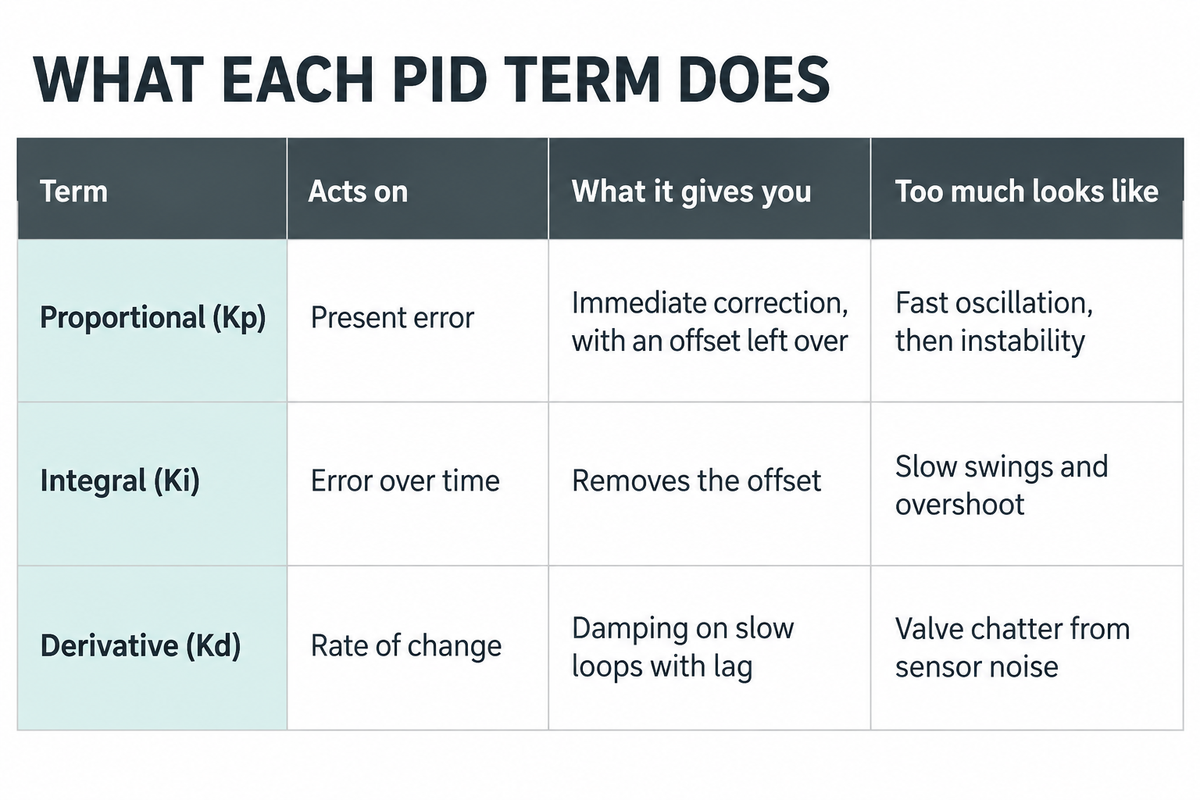
PID tuning is the act of adjusting three parameters so that a control loop’s output brings the process variable to its setpoint quickly and without oscillation; the proportional term responds to the instantaneous error, the integral term to accumulated error, and the derivative term to the rate of change. Control theory combines them into a single equation.
Error is the setpoint minus the process variable (PV), the controlled variable. The controller adjusts the manipulated variable (MV), usually valve position or drive speed, to cut that error. The PID output is the sum of these three terms. The problem is the behaviour of the controlled process, which responds late and by a different amount in every loop.
| Term | Acts on | What it gives you | Too much looks like |
|---|---|---|---|
| Proportional (Kp) | Present error | Immediate correction, with an offset left over | Fast oscillation, then instability |
| Integral (Ki) | Error over time | Removes the offset | Slow swings and overshoot |
| Derivative (Kd) | Rate of change | Damping on slow loops with lag | Valve chatter from sensor noise |
What Are PID Tuning Parameters?
PID tuning parameters are proportional gain (or proportional band), integral time or reset rate, and derivative time. The majority of control systems show just one of each pair, so the initial step on any new controller is to read out which one it actually employs, and in what time unit.
Two conversions cover most blocks. Proportional band is 100 divided by gain, so a gain of 2 equals a band of 50%, and raising the band slows the loop. Integral gain in repeats per minute is 1 divided by integral time in minutes, so raising integral time also slows it. Copying a value without checking these inverts its effect.
ISA technical report TR5.9, released in 2023, names the three algorithm forms in use: parallel, standard and series. With derivative switched off, standard and series behave the same. The parallel form gives each term its own gain, so settings written for standard or series forms need conversion first.
How to Tune a PID Loop in Six Steps
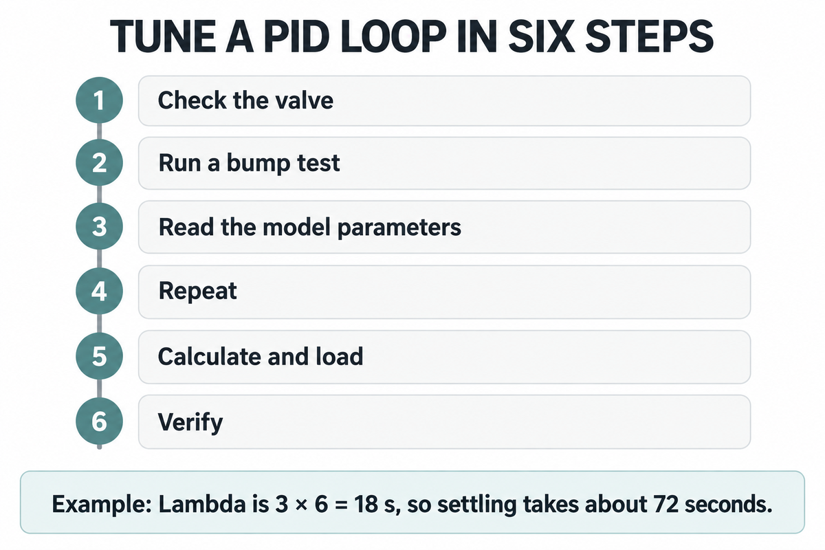
To determine PID settings, confirm the valve moves properly, measure the process with a step test, choose a closed-loop response time, calculate gain and integral time, load the values, and watch the loop for a few days. The following order is valid for self-regulating flow, pressure and consistency loops.
To tune PID controllers on these loops, fit a first order time delay model to the test, which is what steps 2 to 4 produce.
- Check the valve. Step the output by a small amount in manual, both directions, and confirm the PV follows each move.
- Run a bump test. With the loop steady in manual, change the output by a few percent, enough to move the PV about five times its noise band.
- Read the model parameters. Process gain is PV change divided by output change, both in percent of span. Dead time, the time delay, runs from the output step to the first PV movement. The time constant runs from there to 63% of the total change, per Smuts’s lambda notes.
- Repeat. Do two or three more tests and average them, stepping in both directions.
- Calculate and load. Record the old settings with the date, then enter the new ones.
- Verify. Make a small setpoint change, compare the trend with the expected settling time, and watch it for a few days.
Lambda tuning requires one choice from you: lambda, the closed-loop time constant. Guidance in ISA’s InTech for a self-regulating loop is to start at three times the larger of dead time or time constant, which stays stable even if dead time and process gain both double. Then two formulas give the PI settings: Kc = τ / (Kp × (λ + θ)) and Ti = τ, where τ is the time constant, Kp here the process gain and θ the dead time.
Example: a stock consistency loop
Assumed inputs: process gain 1.5, dead time 6 s, time constant 4 s. Lambda is 3 × 6 = 18 s. Controller gain is 4 / (1.5 × (18 + 6)) = 0.11, a proportional band of about 900%. Integral time is 4 s. Derivative is off. Control Engineering pegs settling at about four lambdas, so a setpoint change should be complete in about 72 seconds.
That gain looks small. Dead time limits achievable speed, but settling time also depends on the lambda you choose and the process type. Excessive gain would overshoot or oscillate. Agree the test window with operations first: keeping the old values restores the settings, not a process that drifted during the test.
Level loops are different. A machine chest level won’t settle after a bump; its slope changes. Emerson’s Mark Coughran gives integral time as 2λ + θ for these integrating loops, and Control Engineering puts settling at about six lambdas with some overshoot on a setpoint change. Process gain on these loops is the change in slope divided by the output change; the worked example and worksheet here cover self-regulating loops only.
How Do You Manually Tune a PID Loop?
Manual tuning alters the gains in modest steps in real time to see the response: set Ki as well as Kd to zero, set Kp low, raise it until the action is brisk, then include integral until the offset is gone. Include derivative only where measurement noise is low. The manual tuning method requires no model, yet on a sluggish loop each trial takes a long period of time.
The ultimate-gain form of the Ziegler-Nichols method records the value of Kp at sustained oscillation (Ku) and the period of that oscillation (Pu). Standard course texts take those two readings, and work their settings from them. On a paper machine, manually tuning this way means deliberately cycling a live loop, which can throw off basis weight and every loop downstream; it suits hands-on bench work better than a running sheet, and iterative fine-tuning after a calculated start is the safer use of it.
PID Tuning Methods Compared: Ziegler-Nichols, Cohen-Coon and Lambda
Lambda tuning can be a useful initial method for slow process loops with dead time and for interacting loops. Ziegler-Nichols and Cohen-Coon tuning can produce oscillatory responses, and practitioners often halve the calculated gain to make them less aggressive.
“Lambda tuning is used widely in the pulp and paper industry, where there is a strong connection between paper uniformity and manufacturing efficiency, and control-loop interactions with upstream hydraulics.”
Tim Olsen and Norman Ito of Emerson Process Management, Implement an Effective Loop Tuning Strategy, AIChE CEP, January 2013
| Method | Aims for | Works when | Use it for |
|---|---|---|---|
| Ziegler-Nichols open loop | Quarter-amplitude decay | Time constant at least 2 × dead time | Isolated temperature and gas pressure loops |
| Cohen-Coon | Quarter-amplitude decay | Dead time under 2 × time constant | Self-regulating loops where speed matters most |
| Lambda (IMC for PI) | Chosen response speed; integrating loops can still overshoot a setpoint change | Separate rules for self-regulating and integrating loops; tolerates model error at larger lambda | Paper machine loops, cascades, loops that interact |
The ratio limits come from Jacques Smuts’s practitioner notes, which also rate Ziegler-Nichols as moderately poor on flow and liquid pressure loops and very poor where dead time dominates. Olsen and Ito add that its large gain and short integral time sometimes create process oscillations. Lambda’s weak spot is load recovery: integral time equals the process time constant, so a long time constant means slow recovery from disturbances. Where fast response matters most, Smuts suggests Cohen-Coon with the gain halved.
Same-Loop Tuning Worksheet
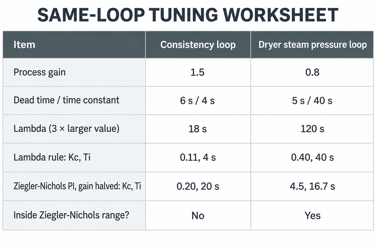
The Same-Loop Tuning Worksheet runs one loop through both rules so you can see how big the disagreement is before touching a controller.
| Item | Consistency loop | Dryer steam pressure loop |
|---|---|---|
| Process gain | 1.5 | 0.8 |
| Dead time / time constant | 6 s / 4 s | 5 s / 40 s |
| Lambda (3 × larger value) | 18 s | 120 s |
| Lambda rule: Kc, Ti | 0.11, 4 s | 0.40, 40 s |
| Ziegler-Nichols PI, gain halved: Kc, Ti | 0.20, 20 s | 4.5, 16.7 s |
| Inside Ziegler-Nichols range? | No, dead time exceeds the time constant | Yes, time constant is 8 × dead time |
For Ziegler-Nichols PI, Kc = 0.9τ / (Kp × θ) and Ti = 3.33θ (from Smuts’s notes, above); on the steam loop the two rules differ by about a factor of 11 in gain, because lambda is deliberately slow. Slower isn’t necessarily better: in this example, reducing lambda to 40 s increases Kc to 1.11 and reduces the estimated settling time from about 480 s to about 160 s. The right tuning is the slowest lambda the process can tolerate; no value is optimal for every grade, and the paper machine section shows what constrains it.
Reducing lambda further has a trade-off. In a simulated temperature loop described by James Beall of Emerson, writing in ISA’s InTech, setting lambda equal to dead time amplified any variability near a 138 second period by 82 percent, a period a poorly performing control valve might produce.
Starting PID Settings for Flow, Pressure, Level and Temperature Loops
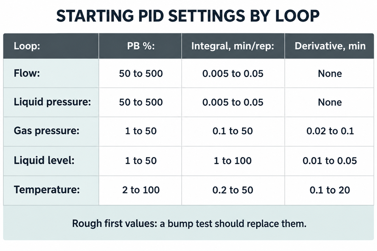
Shinskey’s and McMillan’s initial settings are rough first values for well-designed loops in series or ideal form: flow and liquid pressure with a wide proportional band, short integral and no derivative; level and temperature with a narrower band and longer integral. A bump test should replace them.
| Loop | PB % | Integral, min/rep | Derivative, min | Valve type |
|---|---|---|---|---|
| Flow | 50 to 500 | 0.005 to 0.05 | None | Linear or modified percentage |
| Liquid pressure | 50 to 500 | 0.005 to 0.05 | None | Linear or modified percentage |
| Gas pressure | 1 to 50 | 0.1 to 50 | 0.02 to 0.1 | Linear |
| Liquid level | 1 to 50 | 1 to 100 | 0.01 to 0.05 | Linear or modified percentage |
| Temperature | 2 to 100 | 0.2 to 50 | 0.1 to 20 | Equal percentage |
Valmet’s tutorial credits these values to Shinskey’s Process Control Systems (p.99) and McMillan’s Tuning and Control Loop Performance (p.39). They assume signals scaled in percent of range. Before entering one, check three things on your block: band or gain, minutes per repeat or repeats per minute, and whether the algorithm is parallel. On scaling, ISA’s TR5.9 notes that algorithms using engineering units disrupt tuning methods.
Do You Need Derivative Action, or Is PI Enough?
PI is enough for most flow, liquid pressure and level loops, and the table above lists no derivative at all for the first two. Derivative can earn its place in slower loops with lag and a clean measurement, such as temperature loops, where it can provide phase lead and support a higher gain.
The derivative term reacts to rate of change, so a noisy sensor turns directly into valve movement. If you tune by lambda, Smuts sees little point in derivative at all, since the goal is a calm loop. Olsen and Ito warn that too much derivative in the wrong situation can make a loop unstable. Stock flow on a paper machine sits in the flow row of the table, so leave derivative at zero there and spend the effort on the valve.
PID Tuning on a Paper Machine: Consistency, Headbox, Basis Weight and Steam
On a paper machine, tune each inner loop before the outer loop that drives its setpoint, and separate interacting pairs by five times in lambda. Where basis weight trims stock flow, tune stock flow first; where moisture adjusts steam pressure setpoints, tune steam pressure first. System performance improves when loops stop passing oscillation down the machine.
Lambda is common on paper machines for this reason: it can stop the whole machine oscillating through process interactions. Control Engineering adds that overdamped loops avoid visible irregularities in the finished sheet and spare valves from reversals. Beall gives the two ratios used below: interacting loops should differ in lambda by a factor of five or more, and a cascade inner loop should have 1/5 or less of the outer loop’s lambda.
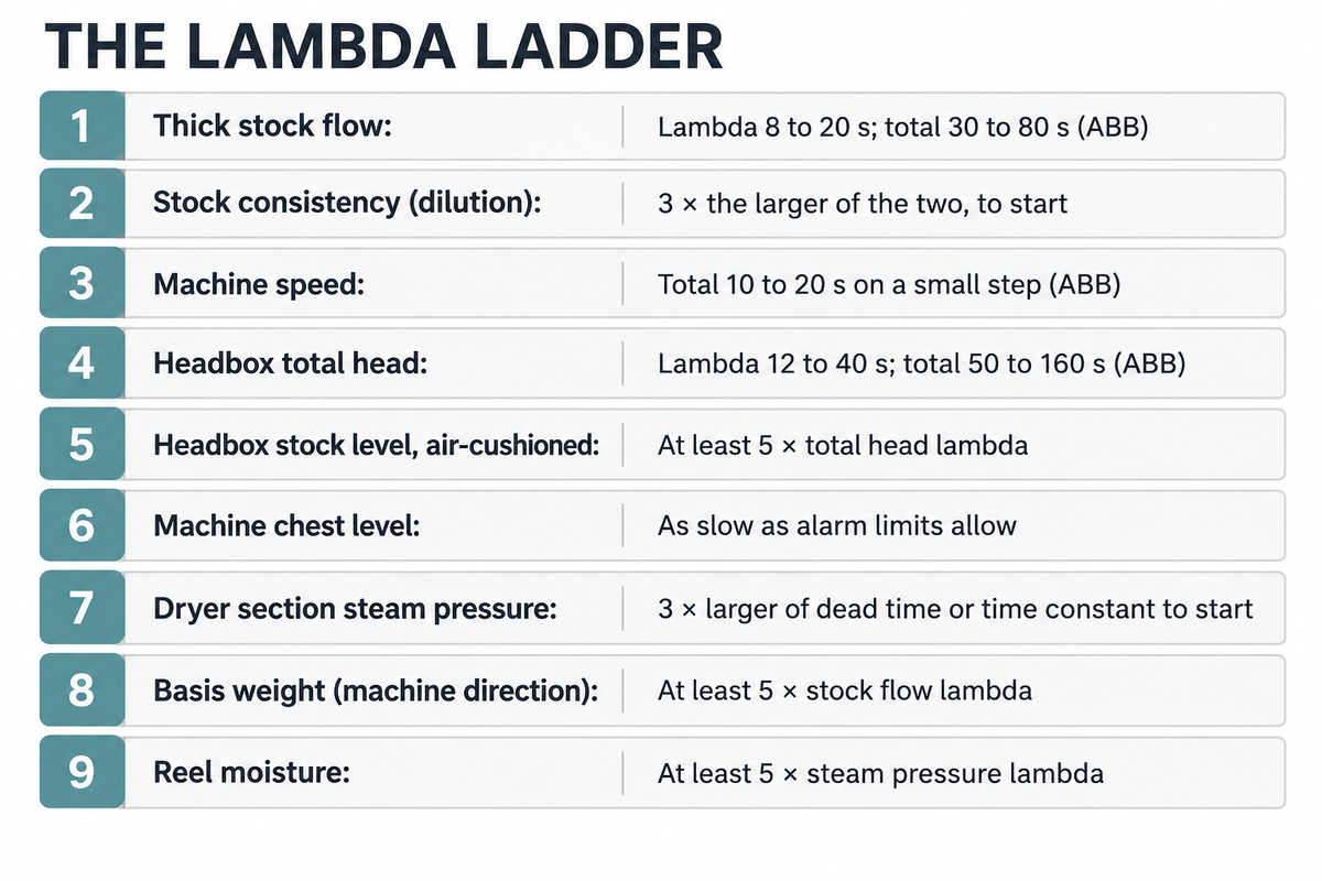
The Lambda Ladder
The Lambda Ladder provides a tune sequence and response target for each paper machine loop. Use the 5-fold separation for each cascade or interacting pair, not between adjacent rows. In an open-loop step test, an integrating chest level changes its slope rather than settling, whereas a self-regulating pipe flow approaches a new value.
| Tune order | Loop | Expected step response | Lambda or response target |
|---|---|---|---|
| 1 | Thick stock flow | First order plus dead time | Lambda 8 to 20 s; total 30 to 80 s (ABB) |
| 2 | Stock consistency (dilution) | First order; measure dead time and time constant | 3 × the larger of the two, to start |
| 3 | Machine speed | Rate limited drive | Total 10 to 20 s on a small step (ABB) |
| 4 | Headbox total head | First order; fan pump is nonlinear | Lambda 12 to 40 s; total 50 to 160 s (ABB) |
| 5 | Headbox stock level, air-cushioned | Integrating, couples with total head | At least 5 × total head lambda |
| 6 | Machine chest level | Integrating | As slow as alarm limits allow; Ti = 2λ + θ |
| 7 | Dryer section steam pressure | First order plus dead time | 3 × larger of dead time or time constant to start |
| 8 | Basis weight (machine direction) | Long dead time: stock travel plus sheet travel to the scanner | At least 5 × stock flow lambda, so 40 to 100 s or more |
| 9 | Reel moisture | Long dead time; moves steam setpoints | At least 5 × steam pressure lambda |
ABB’s numbers are for stock flow, total head and speed. Use the relative rule for consistency and moisture: an interacting pair differs in lambda by a factor of five or more, and a cascade inner loop has 1/5 or less of the outer loop’s lambda.
Stock flow and consistency
In one ABB instance the stock flow loop took 11.4 minutes to react whereas it should have been in the 30-80 second range. On the same machine, automatic grade change commissioning cut transition time from 22.3 minutes (manual) to 15.8 minutes, and also made the stock flow response 10 times faster. A flow loop, which used the position of the valve rather than a meter to infer its measurement, was tuned very slowly and helped sheet weight overshoot its target by 40%.
An IPPTA paper on small mills gives the reason why consistency comes before everything measured at the reel. At 90% overall retention, a one-percentage-point change in retention alters GSM by about 1.1%, with other factors held constant; the same paper estimates a total basis-weight change of the order of 2% or more for a change of 1% in consistency. Good consistency control upstream of pressure screening and through the stock preparation reaches the sheet directly.
Headbox total head and level
Total head has to follow speed changes or the jet to wire ratio slips. ABB suggests a feedforward from the machine speed setpoint to the total head controller, and found that a slow speed loop, 200 seconds versus an expected 10-20, caused the paper machine headbox to rush at the start of a ramp and drag at the end. Look at sectional drives before blaming the total head tuning.
A hydraulic headbox requires one PI controller on total head. Air-cushioned boxes require two, one on total head through the fan pump and another one on level through the air bleed, and a Lakehead University thesis shows that they interact strongly. Separate the two lambdas by five times, and tune the one that matters more for the jet to run faster.
Basis weight without a scanner
A mill with no scanner can still run basis weight control on dry stock flow, which is stock flow multiplied by consistency. The IPPTA authors hold that product constant from a consistency transmitter and a flow meter, with a hand-measured sample every 1/2 to 1 hour. In a trial at 70 gsm and 380 m/min, with a scanner measuring weight continuously and flow set by hand, consistency between 2.75% and 2.85% (IPPTA Table II) was offset by flow settings of 305 and 294, and basis weight held within +1.0% and -0.4% over a shift.
That paper also reported the cost of the system: about Rs 10 lakh for a 60 TPD system in 1996, versus Rs 1.5 to 2 crore for an online scanner at a big mill, with the authors’ stated payback period of about 4 months. Prices are historic, but the ratio accounts for why small mills begin here. Scanner dead time adds up quickly once a scanner is fitted. Assumed inputs: 60 m from slice to scanner at 300 m/min gives 12 s of sheet moving time, before any delay for approach flow.
Dryer steam pressure and reel moisture
Most machines are moisture-controlled via steam. Slätteke’s Lund thesis explains that the moisture controller modifies the setpoints of the steam pressure controllers, resulting in a cascade. Tune the pressure loops first, and keep the moisture five times slower.
Each dryer group in a cascade steam system also holds a differential pressure so that condensate leaves the dryer cylinders. A Valmet Flow Control application note lists 0.4 bar with stationary siphons and 0.8 bar with rotating ones on an example 1200 m/min machine. That loop shares its header with the pressure loop, so the same five-times separation applies. ABB also notes that a large steam change during a grade change can upset the boiler itself, so a setpoint ramp rate belongs in the plan for the paper drying process.
Why an Oscillating PID Loop Is Not Always a Tuning Problem
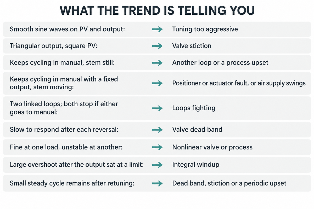
The three common reasons for an oscillating loop are aggressive gain, a sticking/worn control valve, or being driven by another loop. 1993 reports found 20 to 30% of control loops in paper mills oscillating because of valve issues, and those faults remain after any retune, so test before you change a setting.
The 20 to 30% figure, from Bialkowski and Ender as cited in Engineering Applications of Artificial Intelligence, is old and leaves the remaining loops unexplained. A troubleshooting guide in ISA’s InTech gives the test. Put the loop in manual. If the oscillation continues, the source is likely outside the loop, with one exception: a positioner can cycle by itself, so go and look at the valve stem.
| What the trend shows | Likely cause | First action |
|---|---|---|
| Smooth sine waves on PV and output | Tuning too aggressive | Step test, then retune with a larger lambda |
| Triangular output, square PV | Valve stiction | Valve maintenance or positioner tuning |
| Keeps cycling in manual, stem still | Another loop or a process upset | Compare trends to find the likely source |
| Keeps cycling in manual with a fixed output, stem moving | Positioner or actuator fault, or air supply swings | Isolate the valve system before retuning |
| Two linked loops; both stop if either goes to manual | Loops fighting | Make the less important loop 3 to 5 times slower (Smuts, in ISA’s InTech); Beall’s factor of 5 is the safer end |
| Slow to respond after each reversal | Valve dead band | Repair linkage or actuator; tuning cannot fix it |
| Fine at one load, unstable at another | Nonlinear valve or process | Characterize the output, or schedule gains |
| Large overshoot after the output sat at a limit | Integral windup | Set output limits and enable anti-windup |
| Small steady cycle remains after retuning | Dead band, stiction or a periodic upset | Check output, stem travel and linked trends |
One known case: Coughran cites a refinery reactor pressure loop whose as-found tuning resulted in a ±1 psig cycle with a dead band of about 0.7% of output. Applying lambda tuning at 110 seconds eliminated the large cycle, leaving only the small one from the valve. If multiple loops are cycling together, look at their trends; Smuts suggests beginning with the loop that peaks first and looks cleanest, then testing that loop independently.
For the work order, short manual tests provide the proof maintenance needs. Smuts’s checklist lists dead band, stiction, positioner overshoot, oversizing and a nonlinear flow characteristic; he notes that valves are best sized to reach full flow at about 70-90% of travel, since an oversized valve amplifies all the other effects.
Integral windup and anti-windup
Integral windup happens when the output reaches a limit and error continues to exist, so the integral term continues to increase with a good valve already wide open. The loop then overshoots until that stored error unwinds. On a dryer section, look for a steam valve wide open against a short header.
University of Illinois course notes describe the same mechanism. Anti-windup stops the growth. MathWorks documents the two common schemes: back-calculation uses a feedback loop to unwind the integrator, and clamping suspends integration while it would push the output further into saturation. Most modern DCS and PLC blocks already include one, so the check is whether the output limits match what the valve can really do.
PID Tuning Software, Auto-Tuning and Services
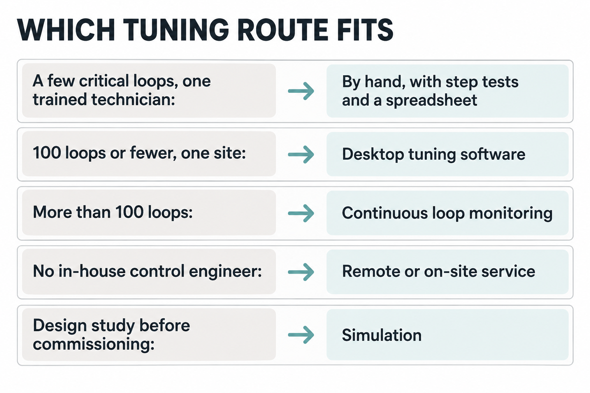
PID tuning software fits a mill with many loops, or relatively little in-house control experience; a small line can tune by hand with the above method and a spreadsheet. Valmet divides its own portfolio at 100 loops: PID Loop Optimizer for 100 or fewer, PlantTriage for more.
| Situation | Option | Examples |
|---|---|---|
| A few critical loops, one trained technician | By hand, with step tests and a spreadsheet | No software cost |
| 100 loops or fewer, one site | Desktop tuning software | Valmet PID Loop Optimizer, Control Station LOOP-PRO |
| More than 100 loops | Continuous loop monitoring | Valmet PlantTriage |
| No in-house control engineer | Remote or on-site service | ABB control loop performance service |
| Design study before commissioning | Simulation | MATLAB PID Tuner, Simulink |
Some of these tools are priced by quotation. One public figure is dated and informal: a February 2020 post to the PLCTalk forum quoted a Control Station toolkit package to existing Toolkit license owners at $1,250 for the first year and $800 for renewals, for what the poster assumed was one basic package.
The benefits most often quoted come from the vendors selling the work. ABB reports that tuning five problem loops at an Indian paper mill cut variability on those loops by 18% to 67%, and managers expecting 10 to 20 percent less product quality variability project $75,000 to $150,000 a year. A Southeast Asian mill with 13 paper machines cut bump test time by 70% and tuning effort by 75%. Use these to set expectations rather than a payback calculation.
Built-in auto-tuning tunes one loop for itself and knows nothing of the Lambda Ladder, so ask what closed-loop speed it produced. For PID loop tuning across a mill, a software tool has value through its real-time trends and records. For system design work, MATLAB’s PID Tuner is used for automated tuning against a plant model with a Bode plot view, and motor teams use the same tools for field oriented control.
Control Scope to Agree on a New or Rebuilt Paper Machine
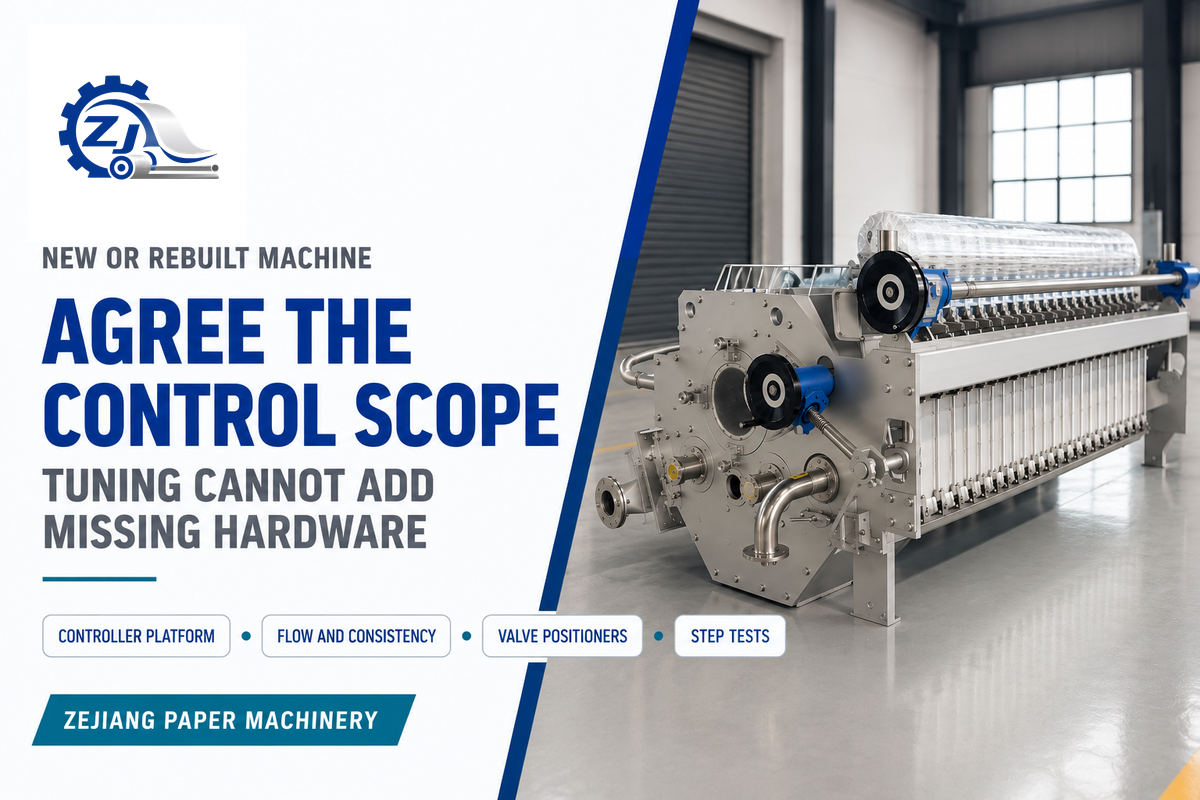
The control scope should identify the controller platform, the actual flow and consistency measurement, the positioners for the critical valves, and who conducts the step tests on start-up. Tuning can’t “add” what the hardware doesn’t have, so these should be included in the quote request, not the punch list.
Each control package is configured per order, from fully manual operation to full PLC control, and our engineering team defines the dryer steam zones and control tuning for each project. Our kraft and corrugated paper machine page lists typical ranges of 1600-5000 mm trim, 30-380 m/min, 10-750 TPD and 70-250 g/m², and that range of grades is exactly what makes a single set of tuning values fall short. We provide direct factory support for installation, commissioning and operator training. Step tests belong in the paper machine commissioning programme, and a paper machine rebuild is the time to bring in those missing meters.
RFQ checklist: copy these into your quote request
| Parameter | Recommended | Why it matters | How to verify |
|---|---|---|---|
| Stock flow measurement | A flow meter on thick stock | Gives measured flow feedback rather than valve position | Meter on the P&ID and instrument list |
| Consistency transmitter | Between machine chest pump and fan pump | Allows dry stock feedforward | Calibration record at start-up |
| Stock flow response | ABB target: total 30 to 80 s | Limits grade change time | Setpoint step recorded at acceptance |
| Total head response | ABB target: total 50 to 160 s | Holds jet to wire ratio during speed ramps | Setpoint step recorded at acceptance |
| Control valve sizing | Full flow at about 70% to 90% of travel | Oversizing magnifies stiction | Sizing sheet from the supplier |
| Tuning records | Final Kc, Ti and lambda per loop | Your team needs a baseline to return to | Handover document |
PID Tuning FAQ
Q: Is a PID controller closed loop?
Yes. A PID controller in automatic runs closed loop, measuring the process and adjusting its output continuously.
In manual the loop is open, and the output stays put, waiting for you to move it. That’s why open-loop step tests start in manual: you can see the process behaviour without automatic controller action mixed in.
Q: Where is a PID controller used?
PID controllers are in use every day across process plants: they run flow, pressure, level and temperature loops; they run motors, heaters and drones.
A paper machine uses them for stock flow, consistency, headbox pressure and dryer steam. The method here works well with these slow process loops, where dead time is a bigger factor than on a servo drive.
Q: Is a PID controller hardware or software?
They both are. Nowadays it’s commonly a software block in a DCS or PLC that executes discrete calculations at a configured interval.
Standalone panel controllers still handle a single heater and small skids. Pneumatic controllers may still be in operation at older plant sites, and Emerson reports tuning them with the same lambda arithmetic as a digital block.
Q: Can I tune a PID controller in real time?
Most systems can accept a change while operating in automatic. Proceed one setting at a time. Record the old setting. Allow about four lambdas between each change, or six if it’s an integrating loop.
Q: Are PID tuning tools worth it?
They’re worth it when you have more loops than one person can test by hand, or when bad tuning is already costing you sheet breaks.
A calculator or spreadsheet will do the same arithmetic as paid software on a clean step test. What you pay for is model fitting on noisy data, diagnostics for valves, and logs of hundreds of loops. Free simulators are useful for practice but won’t show you a sticking valve on your machine.
Q: Does PID tuning work the same on a drone or 3D printer?
They’re the same three terms, but drones run coupled attitude and rate loops, and 3D printers mix motion with slow heater loops. Their handbooks prefer fast trial runs, which don’t often work for a paper machine that’s operational.
Q: Does a PID tuner work with my PLC or DCS?
Offline tuners calculate settings for the controller equations they support; taking live data or writing back settings also requires a compatible interface.
An incorrect form setting results in sensible-looking but poorly behaved values, so check parallel, standard or series first. Data will normally be received by the tool via OPC or an exported trend. On older PLCs with a slow scan, compare the scan time to the dead time of the loop before accepting a fast tuning.
About This Tutorial
Zejiang Paper Machinery manufactures paper machines and pulping equipment in Henan, China. We wrote this tutorial because control tuning determines how well a new kraft or tissue line maintains basis weight and moisture in its first months, and most PID guides end at servo drives and heaters.
References & Sources
- Loop tuning basics: Self-regulating processes, International Society of Automation, InTech
- Loop tuning basics: Complex process responses, International Society of Automation, InTech
- Closed-loop control troubleshooting, International Society of Automation, InTech
- ISA-TR5.9-2023: Realizing and Achieving Best PID, International Society of Automation, InTech
- Implement an Effective Loop Tuning Strategy, AIChE Chemical Engineering Progress, January 2013
- A qualitative shape analysis formalism for monitoring control loop performance, Engineering Applications of Artificial Intelligence
- Basis Weight Control for Small Paper Mills, IPPTA, Vol. 8, No. 3, 1996
- Fundamentals of lambda tuning, Control Engineering
- PID Tuning via Classical Methods, Engineering LibreTexts
- Modeling and Control of the Paper Machine Drying Section, Lund University thesis, abstract